This post will discuss how adding regularization to your machine learning algorithms can improve the accuracy of your algorithm. We will walk through an example of regularization in linear regression, and see how different amounts of regularization impact the accuracy.
Under-fitting and Over-fitting
When we designing machine learning algorithms we risk over-fitting and under-fitting our algorithms. An under-fitted algorithm means simplifying the algorithm too much, to the point where it maps poorly to the data. Over-fitting on the other hand is when you make your algorithm too complex, such that it fits the training data perfectly but fails to generalize.
Examples of under-fitted and over-fitted algorithms are shown below. The under-fitted algorithm is plotted in black and the over-fitted curve is blue.

To address the issue of under-fitting your algorithm you can normally add in more additional features, or make your features of a higher order to better match your data.
To combat over-fitting on the other hand you can reduce the number of features or use regularization. Removing features can be difficult since it is not always clear which features to remove. Regularization on the other hand can easily be applied to your problem by adjusting your algorithm.
Regularization
Regularization in its core will reduce the magnitude of certain θ parameters in our algorithm. Think of it as a damper that will suppress the less useful features in your algorithm, thereby reducing the chance of over-fitting our data. Regularization works best when you have a lot of slightly useful features in your dataset. Slightly useful meaning they may have a lower correlation to the output variable.
To understand how regularization work we will apply regularization to linear regression below. If you not interested in the details you can jump to the example section to see its impact on a real algorithm.
To apply regularization to linear regression we introduce an additional term to our cost and gradient function.
Our regular cost function for a linear regression looks something like this:
\[ \frac{1} {2m} \ \sum_{i=1}^m (h_\theta(x^{(i)}) – y^{(i)})^2 \]
So that is the half mean of the square error.
To apply regularization we introduce a new term controlled by the parameter lambda λ:
\[ \frac{1} {2m} \ \sum_{i=1}^m (h_\theta(x^{(i)}) – y^{(i)})^2 + \lambda\ \sum_{j=1}^n \theta_j^2 \]
Similarly since the gradient function is the partial derivative of the cost function, this also changes the gradient function. The gradient function with regularization is now:
\[ \begin{align*} \newline & \ \ \ \ \theta_0 := \theta_0 – \alpha\ \frac{1}{m}\ \sum_{i=1}^m (h_\theta(x^{(i)}) – y^{(i)})x_0^{(i)} \newline & \ \ \ \ \theta_j := \theta_j – \alpha\ \left[ \left( \frac{1}{m}\ \sum_{i=1}^m (h_\theta(x^{(i)}) – y^{(i)})x_j^{(i)} \right) + \frac{\lambda}{m}\theta_j \right] &\ \ \ \ \ \ \ \ \ \ j \in \lbrace 1,2…n\rbrace\newline & \end{align*} \]
Now since the gradient function is what we use to train our algorithm to the best possible theta values, we can study to the new gradient function to understand what regularization does.
- For \( \theta_0 \) there is no impact – the gradient function remains the same for the offset.
- For \( \theta_j \), that is for every feature term we have the λ term is introduced. This will work to dampen less useful features in your dataset.
As you can see the new parameter λ controls magnitude of our regularization. The optimal value of λ differs from problem to problem. Some machine learning libraries will include functionality to automatically find the best value of λ for your problem and training set.
Example
To test regularization I have generated a few data points using the formula:
\[ y = sin(x) * x \]
Plotted on a XY graph our training data looks like this:
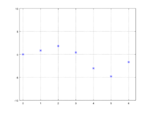
Training data
We will now use linear regression to find a function that best emulates my function. Looking at my training data it is clear that a straight line is not going to be very good at emulating my function. Instead I will have to use a higher order polynomial. To do this I change the input features that I give to my linear regression algorithm from being just [X] to be the following set of features:
\[ \left[ x, x^2, x^3, x^4, x^5, x^6, x^7, x^8, x^9, x^{10}, x^{11}, x^{12}, x^{13}, x^{14}, x^{15} \right] \]
This essentially means that linear regression will find a 15th degree polynomial that fits my training data. This should leave plenty of room for the algorithm to emulate the twists and turns of the sine function, but also leaves us open for the algorithm over-fitting the solution.
First we try to train the algorithm without the use of regularization and plot the resulting function.
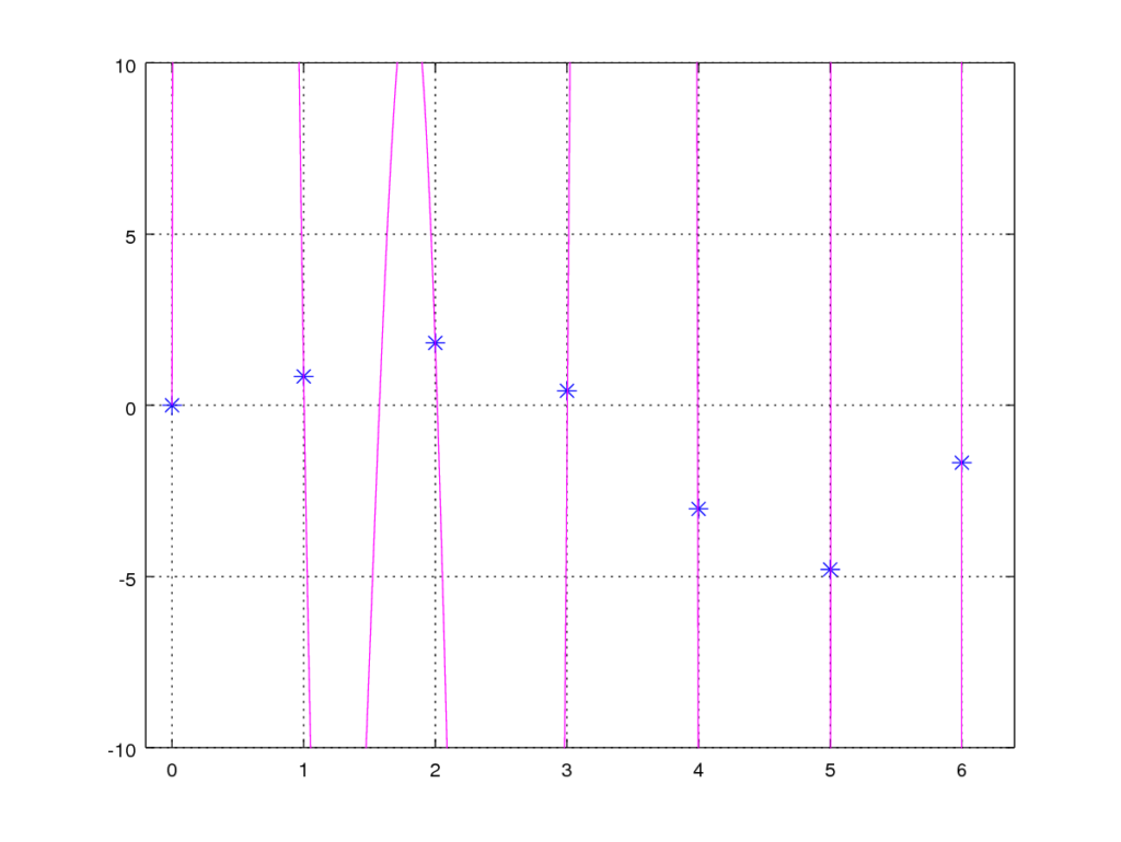
No regularization – λ = 0
With no regularization we see that we found an algorithm that fits the training data perfectly, but the algorithm is terrible at generalizing a solution. For any data that is not in the training set it will gives us the completely wrong result.
At this point we can either try to manually remove input features from the training set to get a better result, or we can use regularization to let the regularization algorithm minimize the impact of the features that are not needed. For our example we try to apply regularization.
With this in mind we try setting λ to 5 and re-run our training.
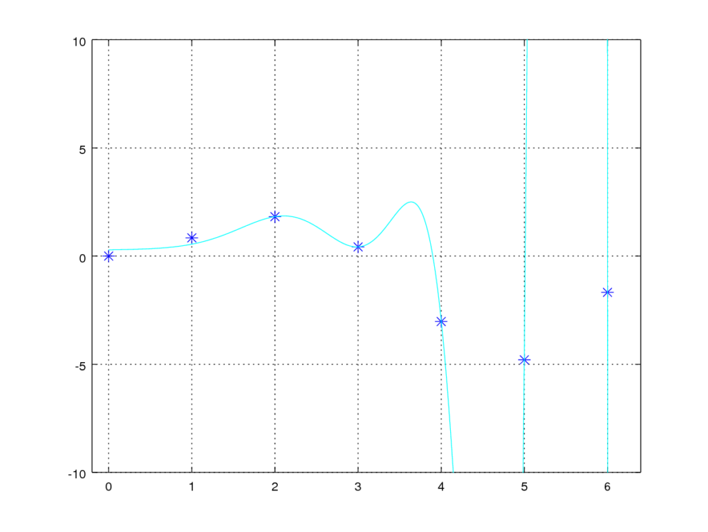
With regularization – λ=5
With λ set to 5 we can see that the resulting function is much better at generalizing a solution. For 0 < x < 3 it gives us a pretty good approximation of the sine function, but it is still not perfect. We therefore try to increase the λ a little bit more. Giving us the following result:
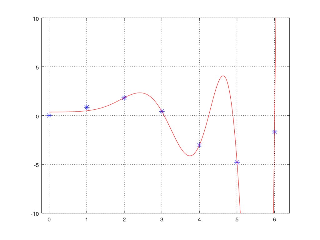
With regularization – λ=13
Having λ set to 13 we find that our algorithm is now getting even better at generalizing a solution for our problem., but unfortunate it is still not perfect at the upper extremes of our training set. While not perfect the model is however still a wast improvement over not having any regularization, This is obviously just an example, in real life we may have used a combination of feature elimination and regularization to get an even better result.
This example showed how applying regularization can wastly improve our machine learning models. Finding the optimal λ value can however be a bit of a challenge. Having one or two dimensional data that allows you to visualize your data makes it a little easier. If you do not have the option to visualize your data I recommend having a solid test data set you can use to calculate your algorithms loss or error. From there you can try a number of different λ values to help you zero in on the one with the lowest error. If you chose this approach, remember that your test data set must be different from your training data – this is only way you can test the generalization of the algorithm and avoid over-fitting your model.
One comment