For this blog post we will walk through how to implement a simple classification algorithm in Ruby using logistic regression. We will use the gem liblinear-ruby to help us setup a model, train it and make predictions in a matter of minutes. For this example we will be using school admissions data to make a prediction on admission based on the result of two exams.
Data
The data we have obtained have 3 rows for each example – the rows contain the following data:
- Result of exam 1 (between 0 and 100)
- Result of exam 2 (between 0 and 100)
- Admission (1 for admitted, 0 if not admitted)
To understand if we can use this data to make predictions we create a XY scatter plot.
Looking at this data we can see that is reasonable to assume we can create a linear model to separate the data. Or said in another way, we can draw a straight line between the two classes of data to separate them and use the line to predict admissions, I’ve added such a line to the plot in green.
A line like this is also called the decision boundary. It can be used for predictions by saying: for anything above the line we predict admission, and below the line we predict the student will not be admitted.
It’s not perfect but its a good start. To calculate where to draw the line we can use logistic regression. The example below will walk you though how to implement this in Ruby.
Implementing Logistic Regression Classification
To get started we want to install the gem called liblinear-ruby. Liblinear-ruby gives us an interface to access the many classification functions from the C/C++ library LIBLINEAR. To install the gem run the following:
gem install liblinear-ruby
Next open an empty Ruby file and start by requiring our liblinear gem and the CSV library.
require 'csv'
require 'liblinear'
Next we load our data from a CSV file into two arrays. One that holds all the exam scores in a two dimensional array (x_data) and one that hold the admitted/not-admitted value (y_data). The exam scores are given as floats and the admitted/not-admitted value is 1 for admitted and 0 for not-admitted.
x_data = []
y_data = []
# Load data from CSV file into two arrays - one for independent variables X and one for the dependent variable Y
CSV.foreach("./data/admission.csv", :headers => false) do |row|
  x_data.push( [row[0].to_f, row[1].to_f] )
  y_data.push( row[2].to_i )
end
For our next step I want to separate our data into two sets. One set to use for training the algorithm and one set to use for testing the accuracy of the algorithm. I’ve decided to allocate 20% of the data for testing and use the remaining 80% for training.
# Divide data into a training set and test set
test_size_percentange = 20.0 # 20.0%
test_set_size = x_data.size * (test_size_percentange/100.to_f)

test_x_data = x_data[0 .. (test_set_size-1)]
test_y_data = y_data[0 .. (test_set_size-1)]

training_x_data = x_data[test_set_size .. x_data.size]
training_y_data = y_data[test_set_size .. y_data.size]
By testing our algorithm with test data instead of the training data we can ensure that the algorithm is not over-fitted. Meaning the algorithm is not trained to match only our training data, but that the algorithm is general enough to also work on data it hasn’t seen before.
At this point we have our data ready and we can initialize a model and train it. We do this in one go when using liblinear like this:
# Setup model and train using training data
model = Liblinear.train(
  { solver_type: Liblinear::L2R_LR },   # Solver type: L2R_LR - L2-regularized logistic regression
  training_y_data,                      # Training data classification
  training_x_data,                      # Training data independent variables
  100                                   # Bias
)
Note I setup my model using the L2 Regularized logistic regression model with a bias of 100. Other models or bias may work better for your specific problem.
Now that we have our model created we can try to make a prediction. We will try to predict if we can get admitted by scoring a 45 on the first exam and 85 on the second exam.
The algorithm works by calculating the probability of our data being in class 1 (admitted) or class 0 (not-admitted). Whichever class has the highest probability will be the predicted class. To inspect these probabilities I will also ask the model to return the probabilities of being in each class. We will output the prediction and the probabilities as a percentage:
# Predict class
prediction = Liblinear.predict(model, [45, 85])
# get prediction probablities
probs = Liblinear.predict_probabilities(model, [45, 85])
probs = probs.sort

puts "Algorithm predicted class #{prediction}"
puts "#{(probs[1]*100).round(2)}% probablity of prediction"
puts "#{(probs[0]*100).round(2)}% probablity of being other class"
For the last step in our sample code will ask the model to make predictions for the data we set aside for testing.
We will compare this prediction to the original class (admitted/not-admitted) for the test data set. This will give us an accuracy of the model we created. We make the predictions and calculate the accuracy like this:
predicted = []
test_x_data.each do |params|
  predicted.push( Liblinear.predict(model, params) )
end
correct = predicted.collect.with_index { |e,i| (e == test_y_data[i]) ? 1 : 0 }.inject{ |sum,e| sum+e }

puts "Accuracy: #{((correct.to_f / test_set_size) * 100).round(2)}% - test set of size #{test_size_percentange}%"
At this point we are ready to run our script. When running on the command line with the following result:
$ ruby example.rb
iter  1 act 2.864e+01 pre 2.469e+01 delta 1.239e-01 f 5.545e+01 |g| 1.556e+03 CG   2
iter  2 act 7.725e+00 pre 6.075e+00 delta 1.239e-01 f 2.681e+01 |g| 4.908e+02 CG   3
iter  3 act 3.153e+00 pre 2.500e+00 delta 1.239e-01 f 1.908e+01 |g| 1.977e+02 CG   3
iter  4 act 9.563e-01 pre 8.030e-01 delta 1.239e-01 f 1.593e+01 |g| 6.458e+01 CG   3
iter  5 act 1.194e-01 pre 1.096e-01 delta 1.239e-01 f 1.498e+01 |g| 1.271e+01 CG   3
Algorithm predicted class 1.0
77.05% probablity of prediction
22.95% probablity of being other class
Accuracy: 85.0% - test set of size 20.0%
The first couple of lines are output from liblinear training our algorithm. Next we see that our algorithm predicted that we would get admitted with a score of 45 on the first exam and 85 on the second, and overall the accuracy of the model when testing with the test data is 85%.
This was how to implement a simple linear logistic regression in Ruby. In the next section we will improve our algorithm by changing the decision boundary from being linear to quadratic.
Improving the accuracy
If we look at our data plot again we can see that maybe a straight line is not the best way of separating the data. Perhaps a curved line would be better as illustrated in blue below.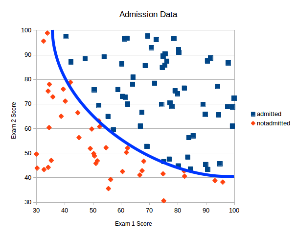
To get a curved decision boundary we need to change the decision boundary function from being linear to some high order polynomial. To test this out we change our data to be second degree polynomial. To do this we change the input data to our logistic regression model. Previously our x_data array contained rows of data like this:
\[ \{ exam1, exam2 \} \]
We change this such that our input instead is a quadratic function like this:
\[ \{ exam1, exam1^2, exam2,exam2^2, exam1* exam2 \} \]
In ruby this means that we change the way we load data like this:
x_data = []
y_data = []
# Load data from CSV file into two arrays - one for independent variables X and one for the dependent variable Y
CSV.foreach("./data/admission.csv", :headers => false) do |row|
  x_data.push( [row[0].to_f, row[0].to_f**2, row[1].to_f, row[1].to_f**2, row[1].to_f * row[0].to_f] )
  y_data.push( row[2].to_i )
end
And we also change our example prediction since it now needs to provide the data in our new format like this:
# Predict class
prediction = Liblinear.predict(model, [45, 45**2, 85, 85**2, 45*85])
# get prediction probablities
probs = Liblinear.predict_probabilities(model, [45, 45**2, 85, 85**2, 45*85])
probs = probs.sort

puts "Algorithm predicted class #{prediction}"
puts "#{(probs[1]*100).round(2)}% probablity of prediction"
puts "#{(probs[0]*100).round(2)}% probablity of being other class"
Executing our script again gives us the following output:
$ ruby example.rb
iter  1 act 8.741e+00 pre 8.341e+00 delta 1.123e-04 f 5.545e+01 |g| 1.561e+05 CG   1
cg reaches trust region boundary
iter  2 act 4.803e-01 pre 4.654e-01 delta 4.491e-04 f 4.671e+01 |g| 1.553e+04 CG   3
cg reaches trust region boundary
iter  3 act 1.403e+00 pre 1.435e+00 delta 1.796e-03 f 4.623e+01 |g| 5.193e+03 CG   3
cg reaches trust region boundary
iter  4 act 2.917e+00 pre 2.853e+00 delta 7.186e-03 f 4.483e+01 |g| 6.573e+03 CG   4
cg reaches trust region boundary
iter  5 act 5.432e+00 pre 5.493e+00 delta 2.874e-02 f 4.191e+01 |g| 3.727e+03 CG   3
cg reaches trust region boundary
iter  6 act 1.495e+01 pre 1.325e+01 delta 1.150e-01 f 3.648e+01 |g| 1.791e+03 CG   4
iter  7 act 3.144e-01 pre 3.067e-01 delta 1.150e-01 f 2.153e+01 |g| 1.866e+04 CG   1
iter  8 act 7.585e+00 pre 5.791e+00 delta 1.150e-01 f 2.122e+01 |g| 1.217e+03 CG   4
iter  9 act 6.789e-02 pre 6.746e-02 delta 1.150e-01 f 1.363e+01 |g| 6.924e+03 CG   1
iter 10 act 4.841e+00 pre 3.640e+00 delta 1.150e-01 f 1.356e+01 |g| 6.975e+02 CG   4
iter 11 act 5.352e-02 pre 5.288e-02 delta 1.150e-01 f 8.722e+00 |g| 2.106e+03 CG   3
Algorithm predicted class 1.0
78.59% probablity of prediction
21.41% probablity of being other class
Accuracy: 95.0% - test set of size 20.0%
By introducing the higher order terms into our data we have increased our accuracy of the algorithm from 85% to 95%.
As you can see finding the correct structure for our input is important – especially for more complex problems that cannot be separated by just a straight line. For more information about how to find the best models and machine learning in general keep coming back to this blog. I will continue to add more posts about machine learning and to solve machine learning problems in Ruby.
To see how you can use a Neural Network to solve this problem and get an even better accuracy check out this blog post.
This technique looks like it only supports binary classification. Could you manipulate the boundary as a closed loop to classify stuff as either inside or outside? I’m thinking in terms of cluster recognition.
Great question! The quadratic function we find in the last part of the blog post is actually a closed loop if we would expand the plot. Generally any polynomial with a higher degree than two will produce a closed loop, and the higher the polynomial the more bends and curves the decision boundary can have.
In terms of binary classification this method can be expanded to classify multiple classes using the one vs all principle (also sometimes called one-vs-rest). See more here: https://en.wikipedia.org/wiki/Multiclass_classification
Hi!
Could you share the csv data set ? Thanks!
Ok, I found it in other post. https://github.com/daugaard/example-neural-network/tree/master/data